Traditionally, mathematics research projects are conducted by a small number (typically one to five) of expert mathematicians, each of which are familiar enough with all aspects of the project that they can verify each other’s contributions. It has been challenging to organize mathematical projects at larger scales, and particularly those that involve contributions from the general public, due to the need to verify all of the contributions; a single error in one component of a mathematical argument could invalidate the entire project. Furthermore, the sophistication of a typical math project is such that it would not be realistic to expect a member of the public, with say an undergraduate level of mathematics education, to contribute in a meaningful way to many such projects.
For related reasons, it is also challenging to incorporate assistance from modern AI tools into a research project, as these tools can “hallucinate” plausible-looking, but nonsensical arguments, which therefore need additional verification before they could be added into the project.
Proof assistant languages, such as Lean, provide a potential way to overcome these obstacles, and allow for large-scale collaborations involving professional mathematicians, the broader public, and/or AI tools to all contribute to a complex project, provided that it can be broken up in a modular fashion into smaller pieces that can be attacked without necessarily understanding all aspects of the project as a whole. Projects to formalize an existing mathematical result (such as the formalization of the recent proof of the PFR conjecture of Marton, discussed in this previous blog post) are currently the main examples of such large-scale collaborations that are enabled via proof assistants. At present, these formalizations are mostly crowdsourced by human contributors (which include both professional mathematicians and interested members of the general public), but there are also some nascent efforts to incorporate more automated tools (either “good old-fashioned” automated theorem provers, or more modern AI-based tools) to assist with the (still quite tedious) task of formalization.
However, I believe that this sort of paradigm can also be used to explore new mathematics, as opposed to formalizing existing mathematics. The online collaborative “Polymath” projects that several people including myself organized in the past are one example of this; but as they did not incorporate proof assistants into the workflow, the contributions had to be managed and verified by the human moderators of the project, which was quite a time-consuming responsibility, and one which limited the ability to scale these projects up further. But I am hoping that the addition of proof assistants will remove this bottleneck.
I am particularly interested in the possibility of using these modern tools to explore a class of many mathematical problems at once, as opposed to the current approach of focusing on only one or two problems at a time. This seems like an inherently modularizable and repetitive task, which could particularly benefit from both crowdsourcing and automated tools, if given the right platform to rigorously coordinate all the contributions; and it is a type of mathematics that previous methods usually could not scale up to (except perhaps over a period of many years, as individual papers slowly explore the class one data point at a time until a reasonable intuition about the class is attained). Among other things, having a large data set of problems to work on could be helpful for benchmarking various automated tools and compare the efficacy of different workflows.
One recent example of such a project was the Busy Beaver Challenge, which showed this July that the fifth Busy Beaver number  was equal to
  . Some older crowdsourced computational projects, such as the Great Internet Mersenne Prime Search (GIMPS), are also somewhat similar in spirit to this type of project (though using more traditional proof of work certificates instead of proof assistants). I would be interested in hearing of any other extant examples of crowdsourced projects exploring a mathematical space, and whether there are lessons from those examples that could be relevant for the project I propose here.
More specifically I would like to propose the following (admittedly artificial) project as a pilot to further test out this paradigm, which was inspired by a MathOverflow question from last year, and discussed somewhat further on my Mastodon account shortly afterwards.
The problem is in the field of universal algebra, and concerns the (medium-scale) exploration of simple equational theories for magmas. A magma is nothing more than a set  equipped with a binary operation
  . Initially, no additional axioms on this operation
  are imposed, and as such magmas by themselves are somewhat boring objects. Of course, with additional axioms, such as the identity axiom or the associative axiom, one can get more familiar mathematical objects such as groups, semigroups, or monoids. Here we will be interested in (constant-free) equational axioms, which are axioms of equality involving expressions built from the operation and one or more indeterminate variables in . Two familiar examples of such axioms are the commutative axiom

and the
associative axiom 
where

are indeterminate variables in the magma
. On the other hand the (left) identity axiom

would not be considered an equational axiom here, as it involves a constant

(the identity element), which we will not consider here.
To illustrate the project I have in mind, let me first introduce eleven examples of equational axioms for magmas:
- Equation1:

- Equation2:

- Equation3:

- Equation4:

- Equation5:

- Equation6:

- Equation7:

- Equation8:

- Equation9:

- Equation10:

- Equation11:

Thus, for instance, Equation7 is the commutative axiom, and Equation10 is the associative axiom. The constant axiom Equation1 is the strongest, as it forces the magma
to have at most one element; at the opposite extreme, the reflexive axiom Equation11 is the weakest, being satisfied by every single magma.
One can then ask which axioms imply which others. For instance, Equation1 implies all the other axioms in this list, which in turn imply Equation11. Equation8 implies Equation9 as a special case, which in turn implies Equation10 as a special case. The full poset of implications can be depicted by the following Hasse diagram:

This in particular answers the MathOverflow question of whether there were equational axioms intermediate between the constant axiom Equation1 and the associative axiom Equation10.
Most of the implications here are quite easy to prove, but there is one non-trivial one, obtained in this answer to a MathOverflow post closely related to the preceding one:
Proposition 1 Equation4 implies Equation7.
Proof: Suppose that obeys Equation4, thus 
for all  . Specializing to
  , we conclude

and hence by another application of
(1) we see that

is idempotent:

Now, replacing

by
in
(1) and then using
(2), we see that

so in particular
commutes with

:

Also, from two applications
(1) one has

Thus
(3) simplifies to
, which is Equation7.

A formalization of the above argument in Lean can be found here.
I will remark that the general question of determining whether one set of equational axioms determines another is undecidable; see Theorem 14 of this paper of Perkins. (This is similar in spirit to the more well known undecidability of various word problems.) So, the situation here is somewhat similar to the Busy Beaver Challenge, in that past a certain point of complexity, we would necessarily encounter unsolvable problems; but hopefully there would be interesting problems and phenomena to discover before we reach that threshold.
The above Hasse diagram does not just assert implications between the listed equational axioms; it also asserts non-implications between the axioms. For instance, as seen in the diagram, the commutative axiom Equation7 does not imply the Equation4 axiom

To see this, one simply has to produce an example of a magma that obeys the commutative axiom Equation7, but not the Equation4 axiom; but in this case one can simply choose (for instance) the natural numbers

with the addition operation

. More generally, the diagram asserts the following non-implications, which (together with the indicated implications) completely describes the poset of implications between the eleven axioms:
- Equation2 does not imply Equation3.
- Equation3 does not imply Equation5.
- Equation3 does not imply Equation7.
- Equation5 does not imply Equation6.
- Equation5 does not imply Equation7.
- Equation6 does not imply Equation7.
- Equation6 does not imply Equation10.
- Equation7 does not imply Equation6.
- Equation7 does not imply Equation10.
- Equation9 does not imply Equation8.
- Equation10 does not imply Equation9.
- Equation10 does not imply Equation6.
The reader is invited to come up with counterexamples that demonstrate some of these implications. The hardest type of counterexamples to find are the ones that show that Equation9 does not imply Equation8: a solution (in Lean) can be found
here. I placed proofs in Lean of all the above implications and anti-implications can be found in
this github repository file.
As one can see, it is already somewhat tedious to compute the Hasse diagram of just eleven equations. The project I propose is to try to expand this Hasse diagram by a couple orders of magnitude, covering a significantly larger set of equations. The set I propose is the set  of equations that use the magma operation at most four times, up to relabeling and the reflexive and symmetric axioms of equality; this includes the eleven equations above, but also many more. How many more? Recall that the Catalan number
  is the number of ways one can form an expression out of
  applications of a binary operation (applied to
  placeholder variables); and, given a string of
  placeholder variables, the Bell number
  is the number of ways (up to relabeling) to assign names to each of these variables, where some of the placeholders are allowed to be assigned the same name. As a consequence, ignoring symmetry, the number of equations that involve at most four operations is

The number of equations in which the left-hand side and right-hand side are identical is

these are all equivalent to reflexive axiom (Equation11). The remaining

equations come in pairs by the symmetry of equality, so the total size of
is

I have not yet generated the full list of such identities, but presumably this will be straightforward to do in a standard computer language such as Python (I have not tried this, but I imagine some back-and-forth with a modern AI would let one generate most of the required code). [UPDATE, Sep 26: Amir Livne Bar-on has kindly enumerated all the equations, of which there are actually 4694.]
It is not clear to me at all what the geometry of will look like. Will most equations be incomparable with each other? Will it stratify into layers of “strong” and “weak” axioms? Will there be a lot of equivalent axioms? It might be interesting to record now any speculations as what the structure of this poset, and compare these predictions with the outcome of the project afterwards.
A brute force computation of the poset would then require  comparisons, which looks rather daunting; but of course due to the axioms of a partial order, one could presumably identify the poset by a much smaller number of comparisons. I am thinking that it should be possible to crowdsource the exploration of this poset in the form of submissions to a central repository (such as the github repository I just created) of proofs in Lean of implications or non-implications between various equations, which could be validated in Lean, and also checked against some file recording the current status (true, false, or open) of all the
  comparisons, to avoid redundant effort. Most submissions could be handled automatically, with relatively little human moderation required; and the status of the poset could be updated after each such submission.
I would imagine that there is some “low-hanging fruit” that could establish a large number of implications (or anti-implications) quite easily. For instance, laws such as Equation2 or Equation3 more or less completely describe the binary operation , and it should be quite easy to check which of the  laws are implied by either of these two laws. The poset has a reflection symmetry associated to replacing the binary operator by its reflection
  , which in principle cuts down the total work by a factor of about two. Specific examples of magmas, such as the natural numbers with the addition operation, obey some set of equations in but not others, and so could be used to generate a large number of anti-implications. Some existing automated proving tools for equational logic, such as Prover9 and Mace4 (for obtaining implications and anti-implications respectively), could then be used to handle most of the remaining “easy” cases (though some work may be needed to convert the outputs of such tools into Lean). The remaining “hard” cases could then be targeted by some combination of human contributors and more advanced AI tools.
Perhaps, in analogy with formalization projects, we could have a semi-formal “blueprint” evolving in parallel with the formal Lean component of the project. This way, the project could accept human-written proofs by contributors who do not necessarily have any proficiency in Lean, as well as contributions from automated tools (such as the aforementioned Prover9 and Mace4), whose output is in some other format than Lean. The task of converting these semi-formal proofs into Lean could then be done by other humans or automated tools; in particular I imagine modern AI tools could be particularly valuable for this portion of the workflow. I am not quite sure though if existing blueprint software can scale to handle the large number of individual proofs that would be generated by this project; and as this portion would not be formally verified, a significant amount of human moderation might also be needed here, and this also might not scale properly. Perhaps the semi-formal portion of the project could instead be coordinated on a forum such as this blog, in a similar spirit to past Polymath projects.
It would be nice to be able to integrate such a project with some sort of graph visualization software that can take an incomplete determination of the poset as input (in which each potential comparison  in is marked as either true, false, or open), completes the graph as much as possible using the axioms of partial order, and then presents the partially known poset in a visually appealing way. If anyone knows of such a software package, I would be happy to hear of it in the comments.
Anyway, I would be happy to receive any feedback on this project; in addition to the previous requests, I would be interested in any suggestions for improving the project, as well as gauging whether there is sufficient interest in participating to actually launch it. (I am imagining running it vaguely along the lines of a Polymath project, though perhaps not formally labeled as such.)
UPDATE, Sep 30 2024: The project is up and running (and highly active), with the main page being this Github repository. See also the Lean Zulip chat for some (also very active) discussion on the project.


. One can then split up a quaternion
and imaginary part
by the familiar formulae
in the complex case).
forming an orthonormal basis). Also, for any
,
is real, hence equal to
. Thus we have a norm
. In particular, the unit quaternions
(also known as
,
, or
) form a compact group.
, together with other familiar formulae such as
,
,
, etc.


 is a double cover of
  .
.

![{[i,j]=ij-ji}](https://s0.wp.com/latex.php?latex=%7B%5Bi%2Cj%5D%3Dij-ji%7D&bg=ffffff&fg=000000&s=0&c=20201002)


does not affect the location
of the tangent vector, but rotates the tangent vector
.
advances the tangent vector by geodesic flow by angle
, and replaces
.


, which corresponds to the operation of replacing a spherical triangle with its dual triangle. Also, there is nothing particularly special about the choice of imaginaries
in (4); one can conjugate (4) by various quaternions and replace
by
for some small
, then we expect spherical triangles to behave like Euclidean triangles. Indeed, (4) to zeroth order becomes
. To first order, one obtains
on the plane, in a suitable asymptotic limit.)


 , while the latter simplifies to
 and
and 


 . Similarly, the second expression simplifies to
 . Equating the two and rearranging, we obtain


 . Meanwhile, the second expression can be rearranged as


 , leading to the “five part rule”
 , this simplifies to one of Napier’s rules
 . The other rules of Napier can be derived in a similar fashion.
of the Sun is positive (due to axial tilt, it reaches a maximum of
at the summer solstice). Then the Sun subtends an angle of
from the pole star (Polaris in the northern hemisphere, Sigma Octantis in the southern hemisphere), and appears to rotate around that pole star once every
hours. On the other hand, if one is at a latitude
, then the pole star an elevation of
, the sun will never set (a phenomenon known as “midnight sun“); but in all other cases, at sunrise or sunset, the sun, pole star, and horizon point below the pole star will form a right-angled spherical triangle, with hypotenuse subtending an angle
, where
is the solar hour angle
) is given by
.


 Hermitian matrix
  whose probability density function is proportional to
  . With this normalization, the famous Wigner semicircle law will tell us that the eigenvalues
  of this matrix will almost all lie in the interval
 ![{[-\sqrt{2N}, \sqrt{2N}]}](https://s0.wp.com/latex.php?latex=%7B%5B-%5Csqrt%7B2N%7D%2C+%5Csqrt%7B2N%7D%5D%7D&bg=ffffff&fg=000000&s=0&c=20201002) , and after dividing by
, and after dividing by  , will asymptotically be distributed according to the semicircle distribution
 eigenvalue
  should be close to the classical location
  , where
 ![{[-1,1]}](https://s0.wp.com/latex.php?latex=%7B%5B-1%2C1%5D%7D&bg=ffffff&fg=000000&s=0&c=20201002) such that
such that 
 defined above, but there are microscopic fluctuations from the classical location that create subtle technical difficulties between “fixed index” results in which one focuses on a single index
  , etc.), and “fixed energy” results in which one focuses on a single energy
 ![{[\delta n, (1-\delta)n]}](https://s0.wp.com/latex.php?latex=%7B%5B%5Cdelta+n%2C+%281-%5Cdelta%29n%5D%7D&bg=ffffff&fg=000000&s=0&c=20201002) for some fixed
for some fixed  , or equivalently the energy
 ![{[-1+c, 1-c]}](https://s0.wp.com/latex.php?latex=%7B%5B-1%2Bc%2C+1-c%5D%7D&bg=ffffff&fg=000000&s=0&c=20201002) for some fixed
for some fixed  . In this region it is natural to introduce the normalized eigenvalue gaps
 have mean close to
 , as well as an exponential decay bound
 , and a lower tail bound
 . We also obtain good control on sums
  of
of  and variance
  . (This is significantly less variance than one would expect from a sum of
  occur in the estimates, which is what one would obtain if one tried to use existing eigenvalue rigidity theorems. (In particular, if one normalized the eigenvalues
  at the same scale at the gap
  ; it is only the gaps between eigenvalues that exhibit much smaller fluctuation.) On the other hand, the dependence on
  is not optimal, although it was sufficient for the applications I had in mind.
 with averaged energy events. For instance, if
  , with the property that there are precisely
  eigenvalues to the right of
  and no eigenvalues in the interval
 ![{[f_x(t), f_x(t+h/2)]}](https://s0.wp.com/latex.php?latex=%7B%5Bf_x%28t%29%2C+f_x%28t%2Bh%2F2%29%5D%7D&bg=ffffff&fg=000000&s=0&c=20201002) , where
, where 

 is the number of eigenvalues to the right of
  is the number of eigenvalues in the interval
  , in particular, affects the distribution of
  , but also the gaps
  of the eigenvalues
  of the top left
  minor
minor  of
of  between the
 is the bottom right entry of
  are complex gaussians independent of
  . This gives a random system of equations to solve for
  . From this, it is possible to leverage the existing universality result of Erdos and Yau to obtain universality of the joint distribution of
  of a fixed number
  of consecutive interlacing gaps
  , where the
  are arbitrary deterministic coefficients. An application of the triangle and Cauchy-Schwarz inequalities, combined with the previous moment bounds on gaps, shows that this randomv ariable has variance
  . However, this bound is not expected to be sharp, due to the expected decay between correlations of eigenvalue gaps. In this paper, I improve the variance bound to
 , which is what was needed for the application.
 . I was not able to establish such decay directly. Instead, using some Fourier analysis, one can reduce matters to studying the case of modulated linear statistics such as
  for various frequencies
  . In “high frequency” cases one can use the triangle inequality to reduce matters to studying the original eigenvalue gaps
  for some increasing sequence
  of natural numbers. Of course, since most real numbers are irrational, one expects such series to “generically” be irrational, and we make this intuition precise (in both a probabilistic sense and a Baire category sense) in our paper. However, it is often difficult to establish the irrationality of any specific series. For example, it is already a non-trivial
  is irrational, while the irrationality of
  (equivalent to
  (
( for any
  can be arbitrarily small positive quantities, which is inconsistent with
  to obtain a rational Ahmes series of growth rate
  for any fixed
  .
.
 , for instance if
  for a fixed
  , then one can find a comparable sequence
  for which
  is rational. This partially addresses
  had this property, and whether any sequence of exponential or slower growth (but with
  convergent) had this property. Unfortunately we barely miss a full solution of both parts of the problem, since the condition
  with
with  such that
  , although the second part (which asks about
  ) is slightly out of reach of our methods. Indeed, we show that the exponential growth hypothesis is best possible in the sense a random sequence
  .
.
 is rational for every rational
  to avoid division by zero)! This answers (in the negative) a question of Stolarsky
  (with the
 . More generally, to represent a tuple of numbers
  indexed by some set
  of numbers simultaneously as
  with
with  , this is the same as asking for the infinite sumset

 be a Banach space, let
  be sets with each
  contained in the ball of radius
  around the origin for some
  with
with  convergent, so that the infinite sumset
  is well-defined. Suppose that one has some convergent series
  in
in  converging in norm to zero, such that
 . Then the infinite sumset
  .
.  “at the scale
  “.
“.
 . Our task is to express
  as a series
  with
with  . From
 and
and  . Iterating this, we may find
  such that
 , we obtain
 are dense enough that the condition
  which will become dense enough to obtain usable inclusions of the form
  reaches the dimension of the ambient space, basically thanks to the inverse function theorem (and the non-vanishing curvatures of the curve in question). For the Stolarsky problem, which is an infinite-dimensional problem, it turns out that one can modify this approach by letting
 is the von Mangoldt function,
  was some suitable approximant to that function,
  was a nilsequence, and
 ![{[x,x+H]}](https://s0.wp.com/latex.php?latex=%7B%5Bx%2Cx%2BH%5D%7D&bg=ffffff&fg=000000&s=0&c=20201002) was a reasonably short interval in the sense that
was a reasonably short interval in the sense that  for some
  and some small
  , and for some other functions such as divisor functions
  for small values of
  ,
,  ,
,  of
of  , that is to say the study of primes in short intervals, until recently the best value of
  , although this was very recently improved to
 and the supremum is over all nilsequences of a certain Lipschitz constant on a fixed nilmanifold
  . This generalizes local Fourier uniformity estimates of the form
 (where, as per the Möbius pseudorandomness conjecture, the approximant
  should be taken to be zero, at least in the absence of a Siegel zero). This is because if one could get estimates of this form for any
  (in particular
  ), this would imply the (logarithmically averaged) Chowla conjecture, as I
  , that is to say prime number theorems in almost all short intervals, until very recently the best value of
  , recently lowered to
  by Guth and Maynard (and can be lowered all the way to zero on the
  in the error terms; for divisor functions, one can even get power savings in this regime.
  , recovering
  , and divisor correlation estimates on arithmetic progressions for almost all
  .
.
 supported on medium scales. So the bad case is when for most
 that depends on
  on
on 
 (and I am being extremely vague as to what the relation “
 ” means here). By a higher order (and quantitatively stronger) version of Walsh’s contagion analysis (which is ultimately to do with separation properties of Farey sequences), we can show that this implies that these polynomials
  (which exert influence over intervals
 ![{[x', x'+Ha]}](https://s0.wp.com/latex.php?latex=%7B%5Bx%27%2C+x%27%2BHa%5D%7D&bg=ffffff&fg=000000&s=0&c=20201002) with some new polynomials
with some new polynomials  and various
  , which are related to many of the previous polynomials by a relationship that looks very roughly like
 and some primes
  with
with  for all
  , then one should have
  for some
  , where I am being vague here about what
  for some
  functions to conclude.
 people, each of which has a probability
  of voting for one candidate, and
  for another… and one can then try to analyze the problem from a dispassionate mathematical perspective. This type of mindset can be illuminating in many contexts. Real world events have real consequences, however, and in light of an event as consequential as the last election, a math lecture on contour integration or the central limit theorem may seem meaningless.
  possible implications between the these 4694 laws.
 implications to resolve,
  have been proven to be true,
  have been proven to be false, and only
  remain open, although even within this set, there are
  implications that we conjecture to be false and for which we are likely to be able to formally disprove soon. For reasons of compilation efficiency, we do not record the proof of every single one of these assertions in Lean; we only prove a smaller set of
  implications in Lean, which then imply the broader set of implications through transitivity (for instance, using the fact that if Equation
  and Equation
  , then Equation
  , which I have nicknamed the “
 ). And here is a
  ; I’ll leave this as a challenge (a four-line proof in Lean is possible).
 in both commutative and non-commutative rings; free magmas associated to “
 and almost all
  , whenever
  is a measure-preserving system (not necessarily of finite measure), and
  ,
,  for some
  with
with  , where
  is a polynomial with integer coefficients and degree at least two. Here we establish the prime version of this theorem, that is to say we establish the pointwise almost everywhere convergence of the averages
 . By standard arguments this is equivalent to the pointwise almost everywhere convergence of the weighted averages
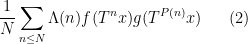
 denotes the
 were “major arc”, at which point this symbol could be approximated by a more tractable symbol. Setting aside the Peluse-Prendiville step for now, the first obstacle is that the natural approximation to the symbol does not have sufficiently accurate error bounds if a Siegel zero exists. While one could in principle fix this by adding a Siegel correction term to the approximation, we found it simpler to use the arguments of Teräväinen to essentially replace the von Mangoldt weight
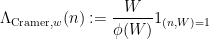
 and
and  is a parameter (we make the quasipolynomial choice
  for a suitable absolute constant
  ). This approximant is then used for most of the argument, with relatively routine changes; for instance, an
  improving estimate needs to be replaced by a weighted analogue that is relatively easy to establish from the unweighted version due to an
  smoothing effect, and a sharp
  -adic bilinear averaging estimate for large
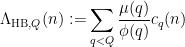
 is the
 , and
, and  in various Gowers uniformity-type norms, which allows us to switch relatively easily between the different weights in practice; hopefully these comparison theorems will be useful in other applications as well.

Recent Comments